Lab 10: Hard Problems and Heuristics

The “Traveling Salesman Problem” is an old and somewhat dated problem in the history of mathematics and computer science. One way in which it’s dated is the gender – everyone can be a salesperson, not just men! Another way in which it’s dated is that “traveling salesperson” is a much less relevant job in this day and age.

What I’ll now call the Traveling Salesperson Problem (TSP) asks us to find the shortest route that allows us to visit a series of locations and then return home. So, you can think of this as a closed loop that includes every location exactly once, except for the starting point (which is visited once at the beginning and once at the end). In graph theory, a loop that visits every location once and returns to its start is sometimes called a tour, and so the TSP asks us to find the shortest possible tour of the locations.

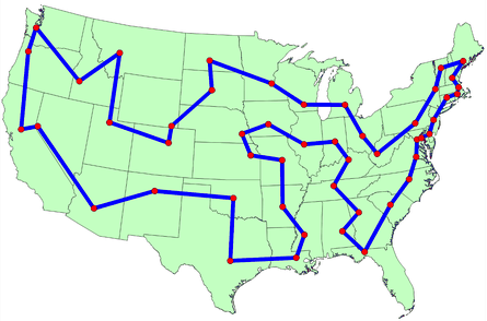
A solution to the TSP for visiting the capitals of the 48 contiguous US states.

Although there are very few actual traveling salespeople anymore, the TSP has a number of applications in engineering and computational science.

The TSP is an example of what’s called an optimization problem. Optimization problems ask us to find a solution to a problem that makes a cost function large or small. In this case, the cost function is the total distance traveled, and we’d like to make that cost as small as possible.

Activity 0

Partnership Planning

Before starting today’s lab assignment, exchange contact information with your partner and find at least two hours in your schedule during which you can meet with your partner to finish the lab. If you are genuinely unable to find a time, please come speak with me!

Reminder: you and your partner are a team! You should not move forward to one activity until you are both comfortable with the previous activity.

Download Starter Code and Data Files

Download this zip file which includes the starter code and data files. Make sure to click extract all if you are a windows user!

The files include:

lab10.py: where you’ll write your lab code!
tsp.py: this file includes some useful functions that you will call in your code.
img/: this isn’t a file, but a folder. The plots that you generate will go here.

Objective

In this lab, you will compare multiple approaches to the TSP in terms of runtime and performance, and use Big-$O$ notation to explain your results.

Our Data

Throughout this lab, we’ll work with randomly generated locations using the random_locations() function that I provided for you. This function accepts a single argument n, which is the number of random locations to be generated. For example, I can generate 5 random locations like this:

locs = random_locations(5)

These locations are stored in a list. Each element of this list is a tuple with two elements, an x-coordinate and a y-coordinate. If you want, you can think of these as latitudes and longitudes.

for loc in locs: 
    print(loc)

(0.41714593276721035, 0.3280831032574511)
(0.4337981635440652, 0.01293283611992346)
(0.9644031013188052, 0.28351704148345425)
(0.9208299217315873, 0.16325776387955515)
(0.24954878352816445, 0.7663845987404052)

Activity 1

Look over how the code so far is structured. There is a function called main() along with:

if __name__ == "__main__":
    main()

As we discussed in class, this means that the main() function will only be called when you run the python script using the green play button in Thonny - no code will run when your functions are imported. This is particularly useful for this assignment, because your code might take a while to run.

The `main()` function

The main() function uses input() to ask the user which activity to run code for (4/7/8/10). You will input the activity number when you get to those activities. You can also input the string "test" to run the test() function. I recommend putting any code that tests that your functions work in the test() function.

Generally, you can’t use input() with the autograder. However, the autograder won’t run the main() function, so this is not a problem as long as you keep the conditional if __name__ == "__main__":.

Your task

In test(), create a variable called locs with 10 random locations using the random_locations() function. Then, write a single expression that gets the y-coordinate (the second coordinate) from the 7th location (the location with index 6). Print both this result and the full list of locations in order to check your answer. Note that the locations are random, so the list will change each time.

Include your code to create locs and find the y-coordinate of the 7th location in test() function.

The Length of a Tour

Now we are going to take steps toward computing the length of a tour.

A distance matrix is a 2-dimensional array of numbers that gives the distance between many pairs of locations. You can calculate the distance matrix for a list of locations using the distance_matrix() function that I have supplied for you in tsp. You use it like this:

locs = random_locations(5)
dists = distance_matrix(locs)

The variable dists is a list of lists. If you want to know the distance between the location with index 1 and the location with index 3, you would check dists[1][3] (or dists[3][1], these are the same).

With the distance matrix in hand, we are ready to compute the length of a tour.

Activity 2

Write a function called total_dist() that accepts two arguments:

seq, a sequence of indices corresponding to locations, provided as a list. For example, the list [4, 1, 0, 3, 2] says “start at the location with index 4, then go to 1, then go to 0, then go to 3, then go to 2, then finish by going back to 4.” Note that the list doesn’t include the “go back to 4” part: that’s implied.
dists, a distance matrix as would be returned by the distance_matrix() function.

The return value of total_dist(seq, dists) should be the total distance traveled in the tour described by seq. In our example above, this would be the sum of the following distances:

The distance from 4 to 1.
The distance from 1 to 0.
The distance from 0 to 3.
The distance from 3 to 2.
The distance from 2 to 4.

Remember that you can get the distances you need using the dists matrix; for example, the distance from 4 to 1 is dists[1][4].

Place your function in the ACTIVITY 2 area of lab10.py.

You are going to need to compute distances between things like seq[i] and seq[i + 1].
You can use a simple for-loop to add together all the distances except the last one (the one that adds the distance for returning to the starting point). You can add that last distance using one additional line of code.

Before moving on, make sure that you’re able to use your function like this:
locs = random_locations(5)
dists = distance_matrix(locs)
seq = [4, 1, 0, 3, 2]

print(total_dist(seq, dists))
You should get a number, although the number you get may be different each time.

This activity is autograded! Submit on gradescope and make sure you are passing the Activity 2 tests before moving on.

Exhaustive Search

Now we’re ready to try our first go at the TSP. To start, we are going to use exhaustive search. Exhaustive search means literally just looking at all the possibilities, computing their distance, and returning the one with the smallest distance.

Activity 3

Write a function called exhaustive_search() that accepts a single argument, locs, a list of locations of the kind that would be returned by random_locations(). It should return two things:

The sequence of indices of locations that achieves the shortest distance.
The shortest distance itself.

To do this, you are going to need to be able to write a for-loop that runs through all possible sequences of locations. Fortunately, there’s a nice way to do that using permutations() from the itertools module:

for seq in permutations(range(n), n):
    ## seq takes on the values of all ways of rearranging the indices [0, 1, 2, ..., n - 1]

If you need to see more about how this works, you might want to try running the below in Thonny:

for seq in permutations(range(4), 4):
    print(seq)

Here’s how I suggest you write the body of this function:
Compute dists, the distances between all pairs of points using distance_matrix().
Initialize a variable best_seq = None and best_dist = 1000000.
For each possible sequence of locations (see above):
Compute the distance associated with that sequence, using the total_dist() function from Activity 2.
If the current distance is less than best_dist, set best_dist equal to the current distance and set best_seq equal to the current sequence.
Finally, return best_seq and best_dist.
NOTE: technically, this implementation is $O(n \cdot n!)$. It turns out that the optimal tour could start at any point (because it is a loop), which means that you only need to consider sequences that start at one point. You can write your code to account for this, but the $O(n \cdot n!)$ solution is acceptable for the purpose of this lab.

You should be able to use your function like this:
locs = random_locations(5)
best_seq, best_dist = exhaustive_search(locs)
print(best_seq)
(4, 1, 0, 3, 2)
print(best_dist)
4.592385
Of course, your numbers are likely to be different because of the random number generation.

This activity is autograded! Submit on gradescope and make sure you are passing the Activity 3 tests before moving on.

Test Exhaustive Search

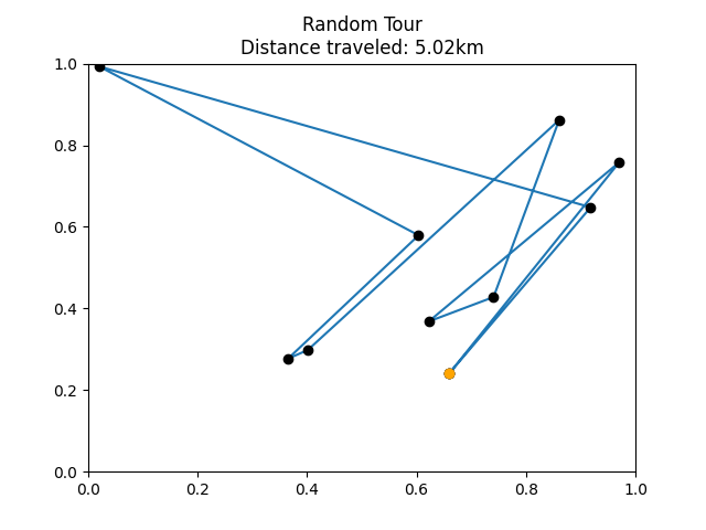
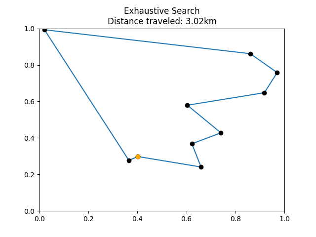
Let’s see if our exhaustive search really works. We can test it by comparing it to a much sillier algorithm that just chooses a totally random path. Here are some examples of what tours might look like:

Example tour visualized from random_tour().

Example tour visualized from exhaustive_search().

Activity 4

By running your script with the green play button and inputting 4, run the code in the elif activity == "4" condition from main(). The code will generate some random locations and then visualize two tours through those locations. The first tour is totally random. The second tour is the optimal route computed using the exhaustive_search() function. After the code successfully runs, plots will appear in the img directory. You’ll eventually turn them in along with the rest of your assignment.

If you are getting a ModuleNotFoundError about matplotlib, use the Thonny Tools –> Manage Packages menu to install the matplotlib module.

Check that you have successfully generated two plots in the img directory and that they qualitatively resemble the examples shown above. You should observe that the distance traveled by the exhaustive_search() tour is significantly lower than the random_tour() tour.

The Greedy Heuristic

Another common term for “exhaustive” search is “exhausting” search, because it’s so slow! Just doing exhaustive search for 10 locations may take several seconds. This is because there are $n!$ possible tours through $n$ locations, and exhaustive search checks all of them. This means that exhaustive search in the TSP has $O(n!)$ runtime. This is extremely bad runtime scaling, and means that exhaustive search is basically unusable for $n$ larger than 12 or so. For example, $15! \approx 1 \; \mathrm{trillion}$, which would take my laptop at least several hours to work through.

What if we have 50 locations to visit? Exhaustive search is simply not an option, and so we may not be able to guarantee that we can find the best tour. This is where we compromise: what if we could find a pretty good tour quickly? Algorithms that give “pretty good” results with practical runtimes are often called heuristics. In the remainder of the lab, you’ll implement the greedy heuristic.¹

Here’s how the greedy heuristic works:

I start out at an initial location.
Then, I move to the nearest location.
Then, I move to the nearest location that I haven’t yet visited.
I continue to move to the nearest location that I haven’t yet visited, until I’ve visited all locations.
Once I’ve visited all locations, I return to my initial location.

First, let’s see if we can learn something about the runtime of this algorithm.

Activity 5

Suppose that I have $n$ locations to visit. How many times do I need to check the distance between two points when running this algorithm? It’s ok to express your answer as a sum rather than in a single formula.

How many distances do I need to look up in order to move from my initial location? How many do I need to look up in order to move from my next location? How many do I need to look up by the time I’ve visited all locations?

Write your answer as a comment in the ACTIVITY 5 area of lab10.py.

Optional challenge: The runtime of the greedy heuristic is $O(n^p)$ for some power $p\geq 1$. Can determine the correct power $p$?

Now it’s time to implement the greedy heuristic.

Activity 6

Write a function called greedy_search() that seeks a tour through a supplied list locs of locations using the greedy heuristic. Your function should return both a sequence of locations and the total distance of the corresponding tour.

Here’s how I suggest you implement this function. I’m assume that there are n locations.
Compute and store the distances between all the locs.
Assume that your starting current location is 0 (we are not trying to find an optimal path, so picking a random starting location is OK). You probably should make a variable to store this information. Create a list called seq that will hold your sequence of locations, and add your starting location to this list.
Make a list of all the locations you haven’t visited yet (to start with, it should be locations 1 through n-1.)
While there are still locations that you haven’t visited yet:
Find the location that has the smallest distance from your current location. Call this location new_loc.
Remove new_loc from the list of locations you haven’t visited yet.
Add new_loc to your seq.
Set new_loc as your current location.
Now you have a seq! Return both the seq and the total distance of the tour (use total_dist() from Activity 2.)

Place your implementation of greedy_search() in the ACTIVITY 6 area of lab10.py.

You should be able to use your greedy_search() function like this, similar to exhaustive_search() from before.

locs = random_locations(10)
seq, dist = greedy_search(locs)

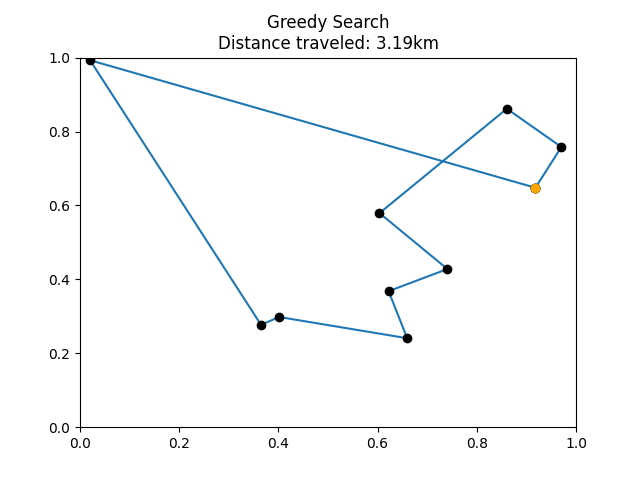
Example tour visualized from greedy_search(), using the same locations as the previous two examples.

This activity is autograded! Submit on gradescope and make sure you are passing the Activity 6 tests before moving on.

Activity 7

Run the code in the elif activity == "7" condition from main(), and take a look at the code to see what it does. You’ll now have three plots in the img directory, visualizing the results for each of the three methods.

In a comment in the ACTIVITY 7 area, describe how greedy search performs in comparison to the random tour and exhaustive search. Is it closer to one or the other?

Timing Comparisons

Based on your analysis and early experiments, you may already suspect that greedy_search() is much faster than exhaustive_search(). How much faster? Let’s check!

Activity 8

Run the code in the elif activity == "8" condition from main(), and take a look at the code to see what it does.

This code will save two more plots in the img directory. The horizontal axis describes the number of locations to be visited, and the vertical axis is the number of seconds that your code took to solve the problem.

In a comment, please compare the runtime of exhaustive_search() and greedy_search() when there are 10 locations to be visited.

Activity 9

Suppose that you wanted to do exhaustive_search with 20 locations to visit instead of 10. The $O(n!)$ scaling implies that exhaustive_search() would require approximately 500 billion times as long to run on 20 locations as it would on 10 locations.

Based on your observation for how long it took your exhaustive_search() to run on 10 locations, estimate the amount of time that would be required to run on 20 locations. Please give your answer in units of years.

According to the musical Rent, there are 525,600 minutes in a year. As you may know, a minute contains 60 seconds.

Activity 10

Run the code in the elif activity == "10" condition from main(), and take a look at the code to see what it does.

You’ll obtain two new plots in the img directory. The first plot generated shows how the time elasped for greedy search depends on the number of locations to search, while the second plot shows an example solution found by greedy search using 201 locations.

Submission

One group member should turn in the file lab10.py and all of the images generated. They should add their partner to the submission.

You should have plots titled:

Exhaustive Search
Greedy Search
Random Tour
Exhaustive Search Times
Greedy Search Times
Greedy Search Times Large
Greedy Search Large

Submit all of these plots on Gradescope alongside your lab10.py file. Nice work!

In Case You Were Wondering…

There are methods that can exactly solve instances of the TSP for several thousand locations in practical time. These methods don’t use exhaustive search; instead, they often use techniques from areas of mathematics called discrete optimization.

The heuristic is called “greedy” because at each step I do the thing that looks best “at the time,” without doing any planning ahead. ↩

Lab 10: Hard Problems and Heuristics

Activity 0

Partnership Planning

Download Starter Code and Data Files

Objective

Our Data

Activity 1

The main() function

Your task

The Length of a Tour

Activity 2

Exhaustive Search

Activity 3

Test Exhaustive Search

Activity 4

The Greedy Heuristic

Activity 5

Activity 6

Activity 7

Timing Comparisons

Activity 8

Activity 9

Activity 10

Submission

In Case You Were Wondering…

The `main()` function